Welcome to my blog

Sentiment Analysis using Scikit-Learn and Model Deployment using Flask and Docker

January 1, 2020

(Imported from my wordpress website)

In this section, we will analyze the sentiments of movie reviews and create a model. Then, we will deploy this model as a REST API using Flask RESTful, and finally create a Docker container for storing this code. The data used can be found here. You can find the full implementation of the code at my gihub page here.

First of all, we will use TF-IDF algorithm and Linear SVC on top of it to analyze sentiments of movie reviews. I have already explained what the TF-IDF algorithm is in one of my previous articles, so take a look at it if you don’t know how it works.

Moving forward, we will deploy our flask model in a python script “app.py”. Let’s import all the required libraries, and create the API using Flask.

Now, we load our models. You can find how they were created here. If you have read my TF-IDF tutorial, it shouldn’t take longer than a minute or two to go through this code.


Now, we create parameters that users can send to this API. These parameters will be stored in a Python dictionary/JSON object. We have added a “query” parameter. This will make a lot more sense when we actually use these parameters, so just hold on.


We use the Resource class to create Flask RESTful APIs. We can also create our methods corresponding to the HTTP requests we need to make. Here, as the user will provide the review, we use a GET request. Then, we store the input and use it to predict the sentiment, as shown.


Now, we add this resource to this API, and run it.


We are done with Flask. Moving on to docker, understand the directory structure first:

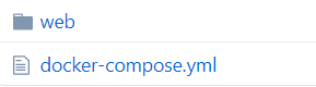Inside the web directory, we have:

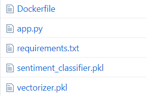We have already discussed how the 2 .pkl model files have been created and the app.py as well. The “web” directory here is essentially one of the services that has been added to this Docker container. Now, we explore the “docker-compose.yml” file.

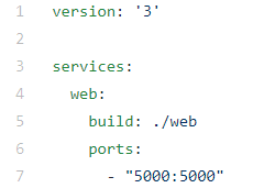Here, as I mentioned just now, “web” has been added as a service to this docker container. We are also saying to build this service from the “./web” directory on our machine, as you can see from the directory structure above, and this service should work at port 5000. Moving on to Dockerfile:

First of all, we will pull the python docker image from DockerHub, which is present here. Now inside this docker container, we set the working directory, and copy the requirements there and install them using pip. Then, we copy all the files from our local machine inside the current directory(“./web”) and we put it into the current working directory in Docker container(“/app”). Finally, we tell docker to run the command(CMD) “python app.py”, which would run our script.

Finally, we take a look at requirements.txt, which will be installed into our Docker container, and are required to run our Python script.

Now, we are ready to build this docker container. If you have already installed docker, open a command prompt and move into the project directory. use the command as shown:

This will display all the docker containers. As we don’t have any yet, it is empty. Now, we build our docker container and this should take some time. This is executing the Dockerfile.

Now, we run our docker container, as follows: 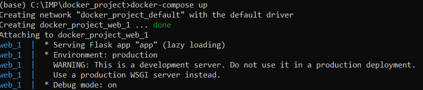If you run the “docker ps -a” command again, you will see the docker container in the list this time. Now, we can make our predictions from our model deployed using Flask:

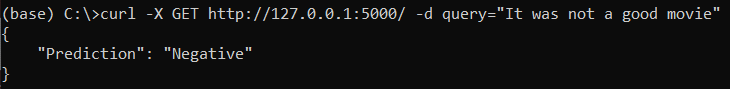Congrats! This surely takes a long time, but model deployment is a part of data analytics just as essential as data collection, preprocessing and modelling.

Finding most popular hashtags on Twitter using Spark Streaming

October 27, 2019

(Imported from my wordpress website)

Spark Streaming is a component of Apache Spark. It is used to stream data in real-time from different data sources. In this section, we will use Spark Streaming to extract popular hashtags from tweets. The complete code implementation in Scala can be found at my GitHub page here.

Working of Spark Streaming can be quickly explained as follows:

1) Streaming Context: It receives stream data as input and produces batches of data.
2) Discretized Stream(DStream): It is a continuous data stream, which the user can analyze. It is represented by a continuous set of RDDs and each RDD represents stream data from a specific time interval. The receiver receives streaming data and converts it into Input DStreams which can be used for processing. Certain transformations can be applied to DStream objects. Output DStreams are used to export data to external databases for storing it.
3) Caching: If the streaming data is to be computed multiple times, it is better to persist it using persist(). It will load this data in memory and by default, data is persisted two times in memory for backup in case of failure.
4) Checkpoints: We create checkpoints at certain intervals to rollback to that point in case of failure in the future.

Let’s begin by importing the libraries:

We need to set up the twitter configuration file. For this, one needs to have a Twitter Developer Account. Go here. Fill the details, create an app, go to details, then keys and tokens and click on regenerate button. We need the API key, API secret key, access token, access secret token to connect to Twitter and stream data.


Creating a StreamingContext which will stream batches of data every one second.


Create a DStream object for Twitter streaming.


Extract hashtags from each tweet.


Now, we will extract hashtags in real-time for 5 minutes, and in a window of 1 second each, we update the count of the hashtags.


Sort the results in descending order.


Set up a checkpoint.


I ran this code in Scala eclipse IDE. After terminating the process, here are the results.

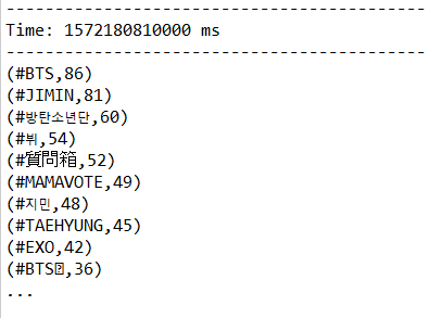As you can see, #BTS was the most popular hashtag during the code execution with a count of 86.

Topic Modeling using Latent Dirichlet Allocation in Scikit-Learn

October 20, 2019

(Imported from my wordpress website)

Topic modeling is used to extract topics with keywords in unlabeled documents. There are several topic modeling algorithms out there which include, one of which will be covered in this section, namely: Latent Dirichlet Allocation(LDA). The complete implementation in Scikit-Learn can be found at my GitHub page here.

Latent Dirichlet Allocation(LDA) is a topic modeling algorithm based on Dirichlet distribution. The procedure of LDA can be explained as follows:

1) We choose a fixed number of topics(=k).

2) Go through each document, and randomly assign each word of document to one of the k documents.

3) Now, iterate over each word in every document.

4) For each word in every document, for each topic t, find:

P(t|d) = Proportion of words in document d that are currently assigned to topic t
P(w|t) = Proportion of assignments to topic t over all documents that come from this word w

5) Reassign each word w a new topic, using:

t(w) = p(t|d) * p(w|t) = Probability that topic t generated word w

Let’s start by importing the libraries and loading data.

As I mentioned, LDA works by assigning a random topic number to each word of the document. So, to tokenize the data, we use CountVectorizer.


Now, we can apply the Latent Dirichlet Allocation(LDA) method.


Now, we can display the results using:


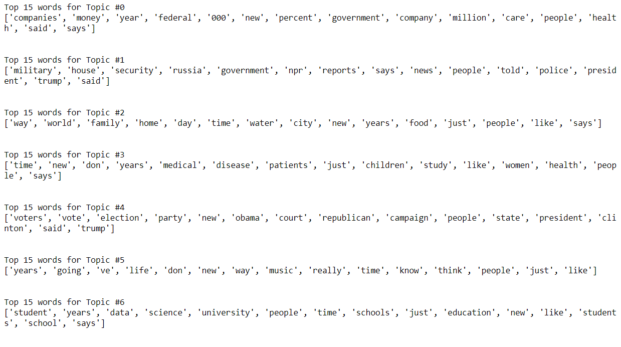Note that LDA is an unsupervised learning algorithm. We did not feed the correct topics to this algorithm, and yet the answers look reasonable. We can also use topic modeling algorithms like Non-Negative Matrix Factorization(NMF or NNMF) for the same purpose.

Feature Extraction using TF-IDF algorithm

October 12, 2019

(Imported from my wordpress website)

The full code implementation along with data used in this section can be found at my GitHub page here.

Suppose we have a document(or a collection of documents i.e, corpus), and we want to summarize it using a few keywords only. In the end, we want some method to compute the importance of each word.

One way to approach this would be to count the no. of times a word appears in a document. So, the word’s importance is directly proportional to its frequency. This method is, therefore, called Term Frequency(TF).

This method fails in practical use as words like “the”, “an”, “a”, etc. will almost always be the result of this method, as they occur more frequently. But of course, they are not the right way to summarize our document.

We also want to take into consideration how unique the words are, this method is called Inverse Document Frequency(IDF).

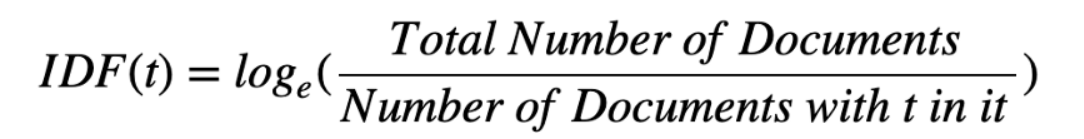So, the product of TF and IDF will give us a measure of how frequent the word is in a document multiplied by how unique the word is, giving rise to Term Frequency-Inverse Document Frequency(TF-IDF) measure.

We implement this using scikit-learn. Let’s begin by reading the file.

Split the data into training and test set.


In scikit-learn, the TF-IDF algorithm is implemented using TfidfTransformer. This transformer needs the count matrix which it will transform later. Hence, we use CountVectorizer first.


Alternatively, one can use TfidfVectorizer, which is the equivalent of CountVectorizer followed by TfidfTransformer


Now, all that’s left to do is use a machine learning algorithm. We can summarize all that we have done so far using a scikit-learn pipeline.


We can find predictions using the predict() method.


To evaluate the predictions, we use different classification metrics.


We have obtained than 99% accuracy in predicting whether the SMS message is spam or ham, and we have performed feature extraction from the raw text in the process.

Web Scraping with Selenium

October 6, 2019

(Imported from my wordpress website)

Data science learners have to spend a lot of time cleaning data to make sense of it before using machine learning algorithms. Being able to collect data is a skill just as important, and a cool one too! In this section, I will explain how to collect data of LinkedIn profiles and store it into MS Excel using Scrapy.

An implementation of this code can be directly found at my GitHub page here.

Assume that your employer wants to hire Python web developers from London. Such tasks can be time-consuming and automating this process can be very useful. I chose Scrapy and Selenium for following reasons:

1) Scrapy is a very fast fully stacked web scraping framework. BeautifulSoup is not as fast and requires more code relatively.

2) Scrapy is not well suited for scraping heavy dynamic pages like LinkedIn. Selenium’s web drivers can make this task very easy for us.

While I could have used the Scrapy framework, for keeping it simple, I have implemented the code using a simple Python script.

Lets start by importing required libraries.

We need to be logged in our own LinkedIn account first to be able to scrape through other LinkedIn profiles. We do this by Selenium webdriver.


The following code will help us extract the urls of LinkedIn profiles we are after.


In this part, we scrape through the required details of each LinkedIn profile, such as name, position, experience, etc.


In this same for loop, we write the code to store this scraped data into our “writer”.


And that’s it! Congrats if you followed till the end, and try to automate your data collection needs using web scraping. It is advisable to not be aggressive while scraping data points(for example, by using sleep() function), else you may get banned.